Machine Learning Zero2Hero with TensorFlow

There’s a lot of hype surrounding AI and Machine Learning, and you’ve probably been inspired by some cool videos that show you what’s possible with these tools. But if we go beyond the hype and write some code, what does Machine Learning really look like?

How We’ll Learn

We’ll be using Python to find out, along with Google’s Tensorflow library for creating Deep Learning models, a category of machine learning that uses multi-layer neural networks.

What is Machine Learning

To understand the theory behind it, let’s start with a basic example of Rock, Paper, Scissors.

Playing this with a human is really basic, and a child can learn to play in just a few minutes. But let’s delve deeper into the most basic part of the game, which the human brain is really good at: recognizing what it’s looking at.

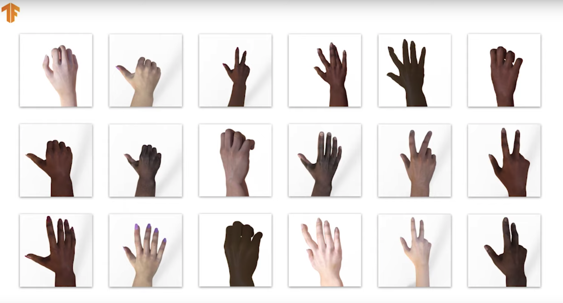
If you take a look at these images, you’ll be able to instantly recognize what each one is. But how would you teach a computer to recognize them? Think of all the diversity of hand types, skin color, or even people who stick their thumb out when doing scissors.

It might take you tens of thousands of lines of code just to play rock, paper, scissors. So what if there was a way to teach a computer to recognize what it sees, or in other words learn in the same way a human does.

This is core to machine learning, and the path to artificial intelligence.

Traditional programming looks like this:

As the programmer, you write rules expressed in a programming language, and feed data to your program to get an answer.
But what if you were to turn this diagram around?

Instead of the programmer figuring out the rules, you give the computer all of the answers along with the data, and let if figure out what the rules are for you.

That’s machine learning!

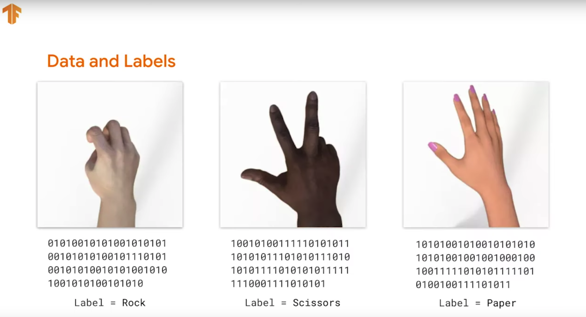
So now I can take lots of labeled images of rocks, papers, and scissors, and tell my computer “this is what they look like.” Then the computer can figure out patterns that match them to each other, and will be able to recognize a rock from a paper from a scissors.

Writing a Simple Neural Network

We’ll start by writing a model for something much simpler. Take a look at these numbers:

X = -1, 0, 1, 2, 3, 4
Y = -3,-1, 1, 3, 5, 7

Can you see the relationship between the X’s and Y’s? It’s:

Y = 2X - 1

But how did you get that? You might’ve looked at the first couple numbers and noticed the Y values were increasing by 2 while X values were increasing by 1, so you knew it was Y = 2X plus or minus something. Then you looked at all of the other numbers and realized that it worked! Recognizing patterns like this is the principle to how machine learning works, and its rough simulation of the human brain is why we call it a neural network.

So we’ll start by importing a couple of libraries that we need:

import tensorflow, keras, numpy as np

Next, we’ll define the model as the simplest possible neural network, which in this case has just a single layer, indicated by the keras.layers.Dense code:

model = keras.Sequential([keras.layers.Dense(units=1, input_shape=[1])])
model.compile(optimizer='sgd', loss='mean_squared_error', metrics=['accuracy'])

It has a single neuron in it, indicated by units=1

We also feed a single value into the neural network, the X value, and will have the network predict what the Y should be for that X, indicated by input_shape being 1 value.

When you compile the model, there are two functions: the loss and the optimizer. These are key algorithms for ML. How it works is:

• The model will make a guess about the relationship between the numbers
• When training, it will calculate how good or bad the guess is, using the loss function.
• It will then use the optimizer funciton to generate another guess
• The combination of these two functions will slowly take us closer to the correct formula.

xs = np.array([-1, 0, 1, 2, 3,4], dtype=float)
ys = np.array([-3,-1,1,3,5,7], dtype=float)

In this case, it will go through that loop 500 times. Our process of matching the Xs to the correct Ys is in the fit function of the model.

model.fit(xs, ys, epochs=500)

What do you think happens when we try to predict the Y when X=10, like so?

print(model.predict([10.0]))

With a relationship of Y = 2X - 1, you’d expect to get an answer of 19. However, the computer was trained to only match 6 pairs of numbers. It looks like a straight line relationship for those six, and while there’s a very high probability that it’s a straight line, we can’t know for certain.

This probability is built into our prediction, and thus we get very close to 19, instead of exactly.

What’s Next

To see and run this code for yourself in a Google Colab, it’s Part 1 of my techranger talk. You can find it and the rest of the 4 parts with the links below:

• Part 1: What you just read!
• Part 2: Basic Computer Vision with Machine Learning
• Part 3: Convolutional Neural Networks
• Part 4: An Image Classifier for Rock, Paper, Scissors

Just hit Open in playground in the top left to open in edit mode and try out the code yourself!

Notes

Credit to Google’s Tensorflow for all images used in this post, adapted from a tech talk I gave at the Center For Distributed Learning.